Data types
Beside of common data types like (Real, Integer, Boolean…) data are combined in a special class record. Record of Soluble and Particulate are defined, where the components are representing the dissolved or particulate components.
record Soluble
  Real O2 "gO2/m3 dissolved oxygen";
  Real I "gCOD/m3 inert soluble organic material";
  Real S "gCOD/m3 readily biodegradable organic substances";
  Real NH "gN/m3 ammonium + ammonia N";
  Real NO "gN/m3 nitrite + nitrate N";
  Real ND "gN/m3 dissolved organic N";
  Real ALK "mol/m3 alkalinity";
end Soluble;
record Particulate
  Real H "gCOD/m3 heterotrophic bacteria";
  Real A "gCOD/m3 autotrophic bacteria";
  Real S "gCOD/m3 particulate slowly degradable substrates";
  Real I "gCOD/m3 inert particulate organic material";
  Real P "gCOD/m3 inert particulate organic matter resulting from decay";
  Real ND "gN/m3 particulate organic nitrogen";
end Particulate;
The use of this records makes the formulation of connectors easier. The data type record can used as component references in expressions
Sini = Soluble(I = 30, S = 1.15, O2 = 4.0,
               NH = 0.2, NO = 10.9, ND = 0.9,
               ALK = 5.5);
Sini can be used as initial condition in the initial equation block.
Functions
Only few functions are formulated. These functions has to adapt to your specified needs.
- Calculation of the saturation concentration of oxygen:
function fS_O2sat
  input Real T;
  output Real S_O2sat;
algorithm
  S_O2sat := exp(7.7117-1.31403*log(T+45.93));
annotation(
  defaultComponentName = "fS_O2sat",
  Documentation(info = "<html>
  <H1 style=\"font-size:20px\">Saturation
      concnetration of oygen </H1>
  <p style=\"font-size:20px\">
  This function determines the saturation
  concentration of oxygen in water aerated
  with air as function of the temperature<br />
  (T in °C S_O2sat in g/m3 at a pressure of 1013 hPa)<br />
  from Mortimer, 1981
  </p>
  </html>"));
end fS_O2sat;
A correlation of the saturation concentration with the temperature is used. The
empirical equation has been adopted from ((Mortimer 1981, eq. 6 page 13)).
Additionally a ß-value can be introduces. The ß-value is the relation between the saturation concentration in the wastewater and the saturation concen-tration in pure water. For municipal wastewater ß is in the range of 0.95 – 1..
- Calculating the volumetric mass transfer coefficient for oxygen
function fkLa
  output Real kLa "specific mass transfer
                   coefficient, 1/d";
  input Real Q "air flow rate, m3/d";
  input Real V_R = 1333 "reactor volume, m3";
  input Real H = 4.5 "fluid height, m";
protected
  Real kLa_stern "-";
  Real v = 10 ^ (-6) "kinematic viscosity
                      of water, m2/s";
  Real g = 9.81 "gravity, m/s2";
  Real w "m/d";
  Real w_stern "-";
algorithm
  w := Q * H / V_R;
  w_stern := w / (84600 * (g * v) ^ (1 / 3));
  kLa_stern := 1.17*10^(-4)*w_stern^(-0.1);
  kLa := kLa_stern * w / (v ^ 2 / g) ^ (1 / 3);
annotation(
defaultComponentName = "fkla",
Documentation(info = "<html>
<H1 style=\"font-size:20px\">kLa calculation</H1>
<p style=\"font-size:20px\">
This function calculates the specific mass
transfer coefficient kLa in '1/d'. The
division by 84600 in the term 'w_stern' is
the conversion from m/d to m/s in order to fit
wwith the units of gravity [m/s2] and viscosity
[[m2/s]. The equations are valid for a gas
distribution systems with perforated bottom,
sintered plate or frite.
Based on
'M. Zlokarnik. Verfahrenstechnische Grundlagen
 der reaktorgestaltung. Acta Biotechnologica
 1, 1981.'
</p> </html>"));
end fkLa;
The main input is the Air flow rate in m 3 /d. The reactor volume in the depth is required as well for the geometry of the reactor. In these case a correlation of Zlokarnik (Zlokarnik 1981) is used, but you may modify this for your need. As well the α value should be considered in this function. The α value is the relation of the mass transfer coefficient for wastewater and pure water. For municipal wastewater α is in the range 0.6 — 1.
3. Sedimentation flux
The sedimentation flux is needed in the secondary clarifier model. The
The sedimentation flux is needed in the secondary clarifier model. The
sedimentation flux is the product of the particle concentration and the
sedimentation velocity. Because the ASM1 is a COD-based model, the solid
concentration is given as COD as well. The sedimentation velocity is calculated as suggested by (Takács 1991). As transformation factor between TSS and COD 0.75 is chosen. For model modification another model for calculation the
sedimentation flux can be introduced.
function fJS "Sedimentation velocity function"
  input Real X "g/m3";
  output Real JS "g/(m2 d)";
protected
  Real v0str, v0 "maximum settling velocity";
  Real nv "exponent as part of the Vesilind equation";
  Real XTSS;
  Real rh, rp;
algorithm
  v0 := 474.0 "m/d";
  v0str := 250.0 "m/d";
  rh := 0.000576 "m3/(g SS)";
  rp := 0.00286 "m3/(g SS)";
  XTSS := X * 0.75;
  JS := min(v0str,
  v0*exp(-rh*XTSS)-
  v0*exp(-rp*XTSS))*XTSS/0.75);
annotation(
defaultComponentName = "fJS",
Documentation(info = "<html>
<H1 style=\"font-size:20px\">Sludge
    Sedimentation Flux </H1>
<p style=\"font-size:20px\">
This function determines the sludge
sedimentation flux according to
Takacs. Input is the concentration of the
particulate components in g COD/m3.
Output in the sludge flux in g COD (m2 d).
</p>
</html>"));
end fJS;
Connectors
Connector are the interfaces between the models (reactor, clarifier …). To distinguish between inflow and outflow two connectors are build (InPipe ![]() , OutPipe
, OutPipe ![]() ). You can imagine that you connect two compartments with a pipe where the water and it’s components flowing to or from a reactor.
). You can imagine that you connect two compartments with a pipe where the water and it’s components flowing to or from a reactor.
connector InPipe
  Real T;
  flow Real Q;
  input Soluble S;
  input Particulate X;
annotation(
Documentation(info = "<html>
<H1 style=\"font-size:20px\">Connector
(for ASM1 components and Flow. Potential
variable is the Temperature </H1>
<p style=\"font-size:20px\">
This connector defines a connector for the
IWA Activated Sludge Model No 1.
For all 13 components as particulate and
dissolved variables and the flow rate. To
fulfill the modelica requirement the
temperature is added as potential variable.
</p>
</html>"));
end InPipe;
The connector OutPipe only differs in the prefix output instead of input . To use these prefixes is required in openmodelica, because variables without prefix are handled as potential variable and require a corresponding flow variable. The modelica handbook Modelica Handbook suggest the stream statement, that you later have to handle with the inStream or actualStream function. This works fine, but is sometimes difficult to explain. In the wastewater model there is a clear direction of transport given and we can use the input and output prefixes. The other advantage is that we can use self defined records for data handling. This saves a lot of code.
Inflow
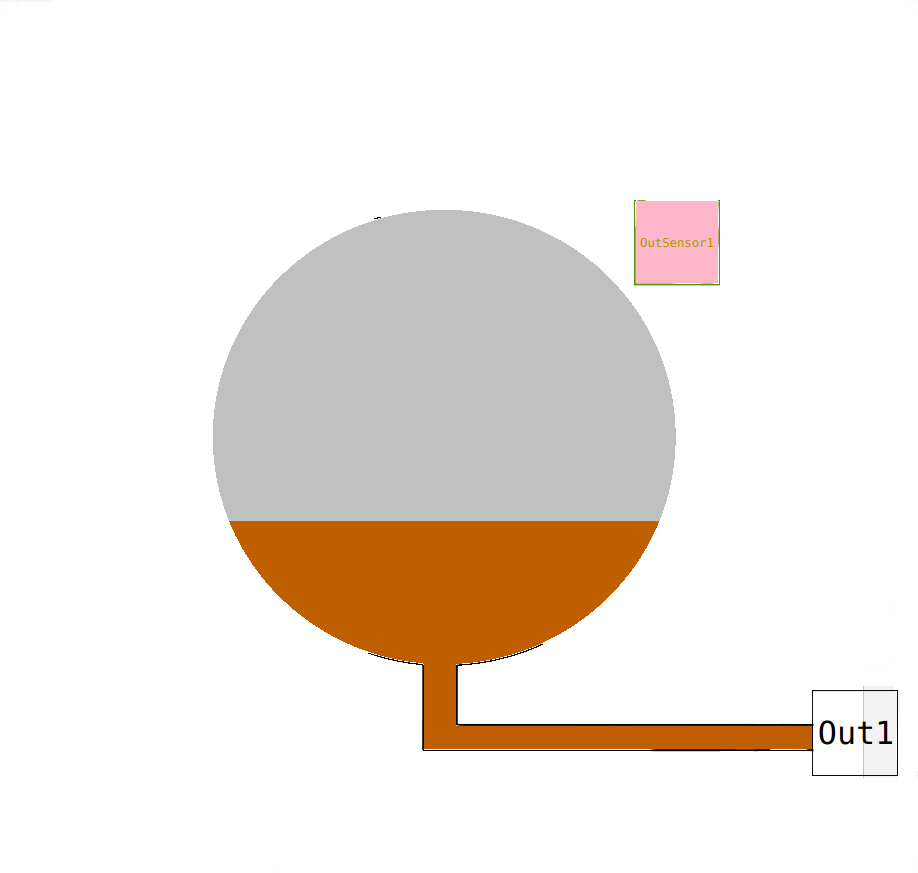
The Infow model delivers the incoming flow rate and the concentration for all components of the model, here 13 components for the ASM1. The temperature is defined here as a parameter. In this package a two Inflow-model are offered, a simple and an advanced model. The simple model Inflow_simple has parameters for the mean concentration of COD, Ntotal, O2 and alkalinity and the flow rate and temperature. In the equation part, the components of the connector Out1 of the type OutPipe were defined. The 7 COD components were multiplied with factors. The sum of these factors should be one. The same is done for the 4 N-components. The alkalinity and the concentration of the dissolved oxygen in the inflow is allocated directly to the Out1 connector element. This simple model is mainly for small models and testing.
In this wastewater model Out1 (and more output Out2, Out3,,,) for the OutPipe connector type. Out1 is the main flow. The same is done for the InPipe connectors (In1, In2, In3..)
The more advanced inflow model in call Inflow. It has only two parameters, temperature and a String variable Inf_File that contain the path and file name of the data for the inflow. Some examples you can find in the sub-directory Resources/ASM1 of the wastewater package. You can find data for the inflow after primary sedimentation, according the the model of the COST Action 624 for dry, rain and storm-weather conditions. For the raw wastewater inflow these file have the name Raw included.
model Inflow "inflow ASM1"
  …
  parameter String inf_file = "/PATH/Inf_dry.txt";
  Modelica.Blocks.Sources.CombiTimeTable T_data(
    tableOnFile = true,
    fileName = inf_file,
    smoothness = Modelica.Blocks.Types.Smoothness.ContinuousDerivative,
    extrapolation = Modelica.Blocks.Types.Extrapolation.Periodic,
    tableName = "t_data",
    columns = {2,3,4,5,6,7,8,9,10,11,12,13,14,15},
    startTime = 0.0);
  OutPipe Out1;
equation
  Out1.S.I = T_data.y[1];
  …
  Out1.Q = -abs(T_data.y[14]);
  Out1.T = T;
end Inflow;
Formate of the data file
\#1
double t_data(5,4)  # t S_S X_H     Q
0   63.63455    0   21477
0.010416667 61.67313    0   21474
0.020833333 61.71973    0   19620
0.03125 62.16018    0   19334
0.041666667 64.57526    0   18978
The first line always starts with a #1 to indicate the type of the file. The second line starts with the data type in c-notation (float, double) followed by the name of the table. (number rows,number cols) after # comment. More than one table can stored in one file. Each table starts in this way. The next rows contain the data where the columns are separated by spaces, tab (\t), comma (,), or semicolon (;). The decimal delimiter is a point (.) The first column contains the time (in this model in days [d]), the next columns the data. To read the data in modelica, a modelica instance of the Modelica.Blocks.Sources.CombiTimeTable is defined (here called T_data). The parameter of this model are:
- tableOnFile: Boolean variable true is the table in a file, false if the table is included in the model.
- smoothness: Integer that gives the form of interpolation; for better understanding the modelica class Modelica.Blocks.Types.Smoothness is used.
1 LinearSegments: linear interpolation
2 ContinuousDerivative: smooth interpolation with Akima-splines such that der(y) is continuous, also if extrapolated.
3 ConstantSegments: constant segments
- extrapolation: Interger that give the form of extrapolation; for better understanding the modelica typeModelica.Blocks.Types.Extrapolation is used.
1 HoldLastPoint: hold the first or last value of the table, if outside of the table scope.
2 LastTwoPoints: extrapolate by using the derivative at the first/last table points if outside of the table scope. (If smoothness is LinearSegments or ConstantSegments this means to extrapolate linearly through the first/last two table points.).
3 Periodic: periodically repeat the table data (periodical function).
4 NoExtrapolation: no extrapolation, i.e. extrapolation triggers an error. - tableName: String with the name of the table (here t_data)
- columns: a list of integer for the columns used {2,3,7} T_data.y[1] refers to the second column, T_data.y[2] to the third column and T_data.y[3] to the seventh column
- startTime: is an offset of time. The time in the table is interpretated relative to the startTime
- offset: is an offset of the ordinate, all values are relative to the offset
- timeScale: if the time in the table has a different unit than your model you can use this factor to for conversion.
There are some more option, please refer to the description of the block CombiTimeTable. OpenModelica 13.2 give some Symbolic Warning for not using all parameters, but you can ignore this. The values are stored in the variable y as a vector. Please remind that outgoing flows are negative. To ensure this the negative absolute value of the flow variable is connected to the Out1.Q (Out1.Q = -abs(T_data.y[14]);)
The Inflow model has two output connector, Out1 (Outpipe) and OutSensor1 (outWWSensor). The Out1 you can connect with the In1 of another model. The OutSensor1 is used for control purpose, and can, no necessarily connected to a controller.
Primary clarifier
The primary clarifier model base on ideas from Otterpohl and Freund, 1992, and is realised as an dynamic model. The retention behaviour is modeled as a cascade of 6 CSTR’s. Therefore the parameter V (volume) is required. The input to the pre-clarifier model (PreClar) is realised with a InPipe connector In1. The distribution of the flows is done by the sub-model PreThick. There the separation of solid occurs depending on the hydraulic retention time with an empirical formula. The dissolved components are not separated. The degree of separation for the particulate components is calculated and the concentration of the treated water phase is calculated (Out1.X. = (1-n_X)*In1.X.) for the six particulate components. The concentration of particulate components in the sludge flow, is calculated with a mass balance (Out2.Q * Out2.X. + In1.Q * In1.X. + Out1.Q * Out1.X. = 0;) and depend on the flow rate. The output connector Out2 has to be connected to a pump, to provide the flow rate Out2.Q.
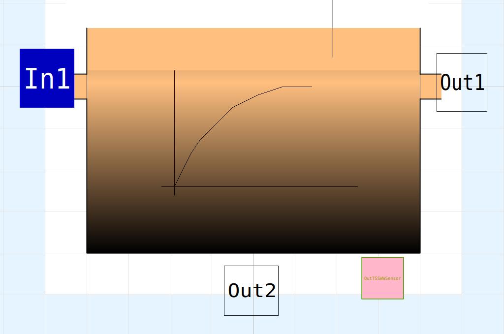
The primary clarifier model has a outWWSensor (OutTSSWWSensor) connector. This signal can be used to control the sludge flow rate (Out2.Q) with the pump. A simple PI-controller can adjust the sludge concentration of the thickened primary sludge. An example can be found in the part TechUnits.SludgeControl.
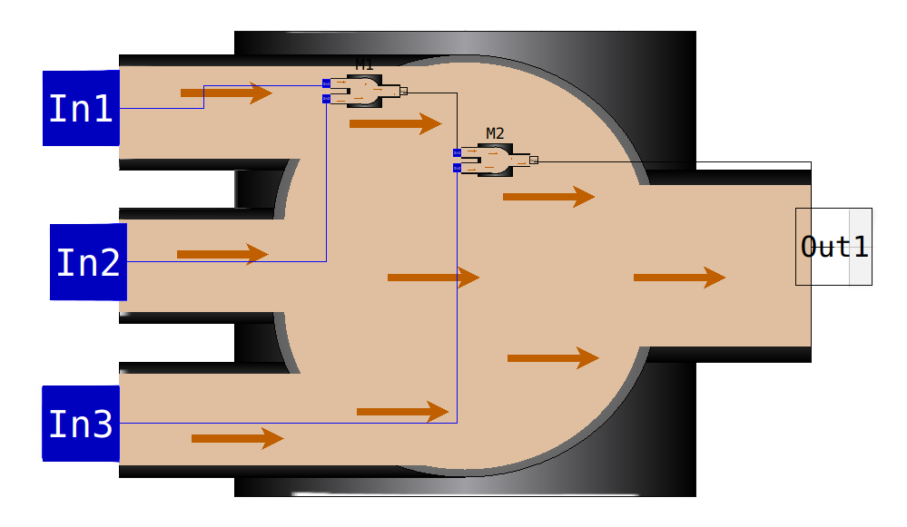
Mixer
In this package two mixer models are offered (Mixer2 and Mixer3). The connectors of the type InPipe, In1, In2 etc. were mixed. The outflow is the negative sum of all inflow rates. The temperature from In1.T is directed to the Out1.T. For all 13 components mass balances were used to calculate the outflow concentrations.
Divider
The divider divides one flow in two flows. The InPipe connector In1 is dividest to the OutPipe connector Out1 and Out2. The Temperature In1.T is set for both Out1.T and Out2.T. The flow rate Out2.Q has to be integrated for another source, like a Pump that is connected with Out2.
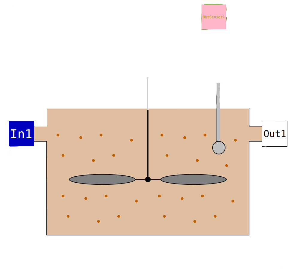
ASM- Rectors
With in this package the Activated Sludge Model No 1 ASM1 is used. This should initiate further developments (ASM2d, ASM3, P-Prec., …). The core of the reactors is the model ASM1_CSTR. It has one InPipe connector In1 and one OutPipe connector Out1. The only parameter is the rector Volume V_R. A sensor OutSensor1 is attached as well. The class kinetic is included with the extends statement to have access to the kinetic parameters. The partial model WWParameters is extended to have access to the classical wastewater parameters. The 8 process rates from ASM1 were defined r1 – r8 and the aeration rate rA.The the 13 mass balances for all components are formulated. This partial model is used for the defination of the NitrificationTank model and the DenitrificationTank model. Beside of the different icons the volumetrik mass tranfer coefficient has to be defined. For the DenitrificationTank model this is realised with a parameter kLa. The NitrificationTank model needs aeration. Therefore a InQ connector InQair is introduced. For the calculation of the kLa value the high of the reactor is required and implemented as a parameter. The volumetric mass transfer coefficient is than calculated with the function fkLa.

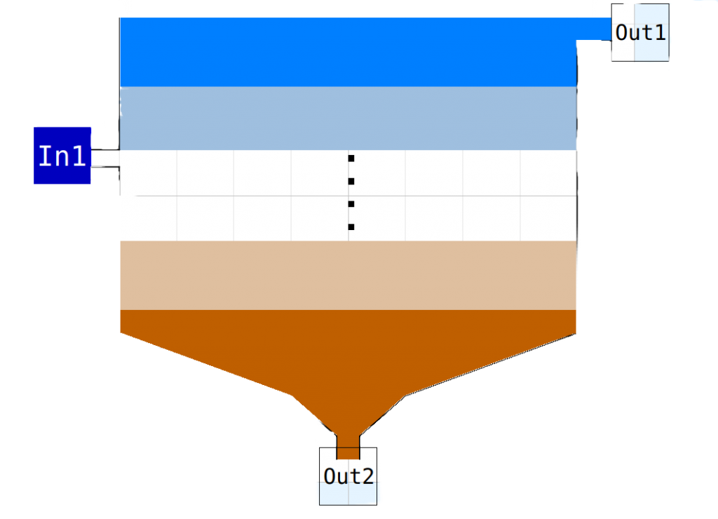
Secoundary Claritier
The secondary clarifier model is in the sub-package SecClar and has the name SCL. The model is a layer based model. the inflow in directed to the fifth layer and split into two flows. The clear water to four layers above and the sludge flow to five layers below. The sedimentation flux is directed to the layers below. The model has three parameter:
A: superficial surface for sedimentation in m2
z: height of one layer of 10 in m
fns: fraction of not sedimentable soldis
The model has one InPipe connector In1 and two OutPipe connectors Out1 for the clear water and Out2 for the sludge. The flowrate of the sludge has to be given by a pump, optionally with a divider and two pumps.
Technical Units
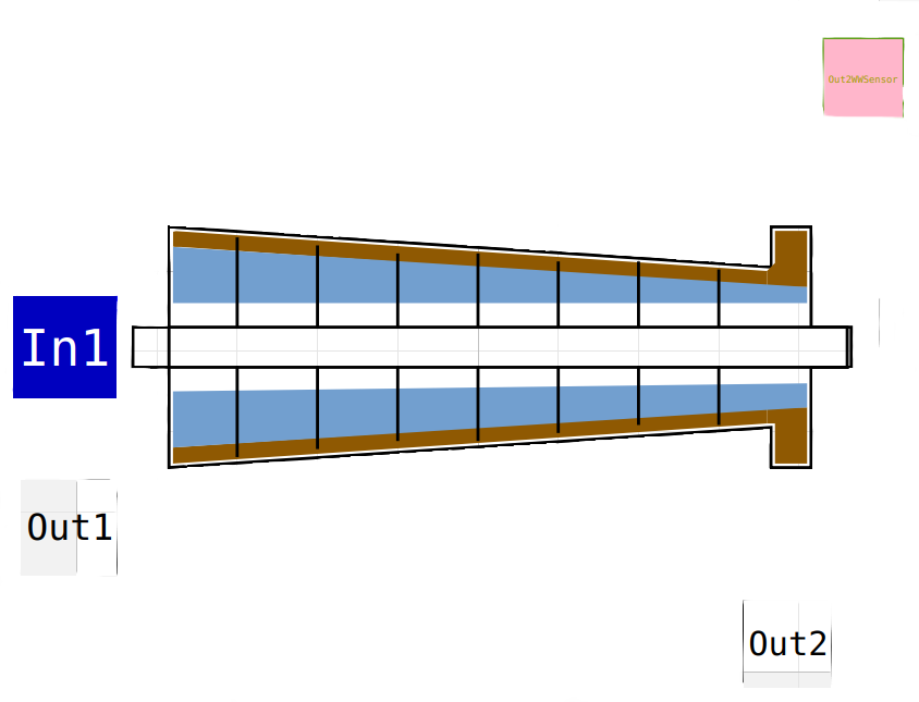
Centrifuge
The Centrifuge model has a InPipe connector In1 and two OutPipe connector Out1 for the water and Out2 for the sludge. The flow rate for the sludge has to be transmitted via a pump. In the sludge flow a outWWSensor connector is defined. This connector can be used for controlling the sludge flow.
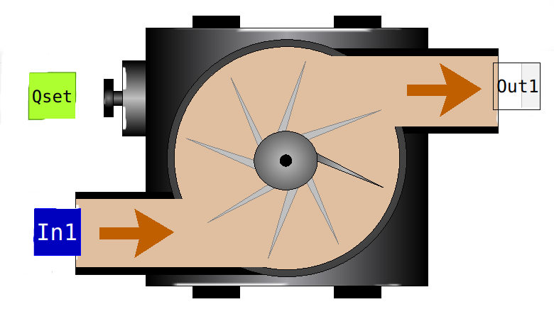
Pump
A pump transport the wastewater components with a flow rate. The model is to be connected with in InPipe (In1) and Outpipe (Out1) connector. The flow rate set point is given bei the Real input Qset. With a given time constante k_DT (default value 5.0 1/d) the flow rate of the pump is reaching the setpoint flow rate. Two other parameter are used for the characterisation of the pump (Qmax and Qmin in m3/d) what is self explaining.
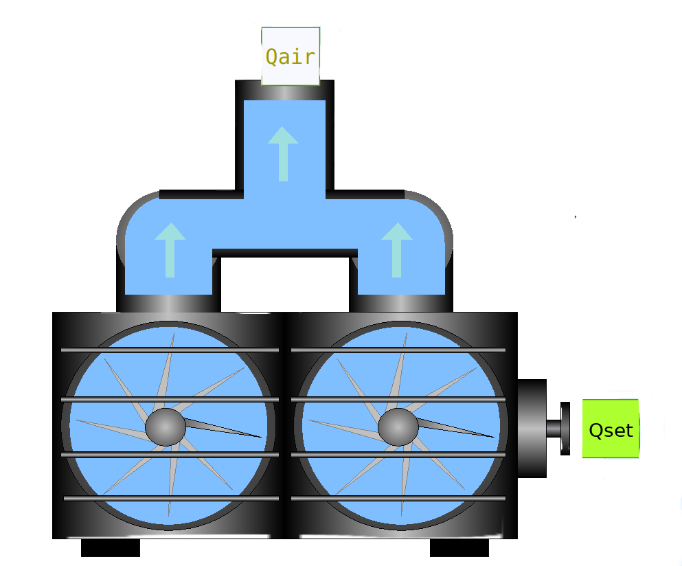
Blower
The Blower connector servers to give the air flow rate information to the NitrificationTank where this flow rate is used to calculate the volumetric oxygen mass transfer coefficient kLa. The model has three parameter, the maximum air flow rate (Qmax) the minimum air flow rate (Qmin) and the response time constant (k_RT). The inQ connector Qset gives the wanted air flow rate. With respect to the the time constant the the the outQ connector Qair the Qair.Q is calculated. Defaul value for k_RT is 50 d-1
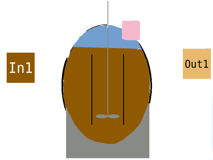
Anaerobic Digester Model
Description of the ADM
Literuture
Batstone, D.J., J. Keller, I. Angelidaki, S.V. Kalyuzhnyi, S.G. Pavlostathis, A.
Rozzi, W.T.M. Sanders, H. Siegrist, and V.A. Vavilin. 2002. “The IWA
Anaerobic Digestion Model No 1 (Adm1).” Water Science and Technology 45
(10): 65–73. https://doi.org/10.2166/wst.2002.0292.
Copp, J. B, European Commission, Directorate-General for Research, and EC.
COST Action 624: the COST simulation benchmark. Description and
simulation manual. Luxenbourg: Office for Official Publications of the
European Communities. https://publications.europa.eu/en/publication-
detail/-/publication/8448ef88-37dd-4d1a-823f-3143e7902429.
Copp, John B. 2001. The COST Simulation Benchmark-Description and
Simulator Manual. COST, European Cooperation in the field of Science and
Technical Research.
https://www.cs.mcgill.ca/~hv/articles/WWTP/sim_manual.pdf.
Henze, Mogens, ed. 2007. Activated sludge models ASM1, ASM2, ASM2d and
ASM3. Reprinted. Scientific and technical report / IWA 9. London: IWA Publ.
Liedke, Moritz. 2017. Development of a wastewater treatment plant model
including sludge treatment with OpenModelica. Master Thesis at TUHH,
Istitute of Wastewater Management and Water Protection.
Mortimer, C. H. 1981. “The Oxygen Content of Air-Saturated Fresh Waters over
Ranges of Temperature and Atmospheric Pressure of Limnological Interest:
With 6 Figures and 1 Table in the Text and on 1 Folder, and 4 Appendices.”
SIL Communications, 1953-1996 22 (1): 1–23.
https://doi.org/10.1080/05384680.1981.11904000.
“OpenModelica User’s Guide.” n.d. Open Source Modelica Consortium. Accessed
January 12, 2022.
https://www.openmodelica.org/doc/OpenModelicaUsersGuide/OpenModelic
aUsersGuide-latest.pdf.
Otterpohl, R., and M. Freund. 1992. “Dynamic Models for Clarifiers of Activated
Sludge Plants with Dry and Wet Weather Flows.” Water Science and
Technology 26 (5-6): 1391–1400. https://doi.org/10.2166/wst.1992.0582.
Reichl, Gerald, Horst Puta, Manfred Köhne, and Martin Otter. 2006. Optimierte
Bewirtschaftung von Kläranlagen basierend auf der Modellierung mit
Modelica. 1. Aufl. Göttingen: Cuvillier.
Takács, I. 1991. “A Dynamic Model of the Clarification-Thickening Process.”
Water Research 25 (10): 1263–71. https://doi.org/10.1016/0043-
1354(91)90066-Y.
Zlokarnik, M. 1981. “Verfahrenstechnische Grundlagen der Reaktorgestaltung.”
Acta Biotechnologica 1 (4): 311–25. https://doi.org/10.1002/abio.370010402.
1391-1400